3 Compute the connectance

The connectance is one of the properties characterizing a network and is defined as the ratio between the actual number of links (i.e. pairwise interactions among species) and the maximal number of links that could be realized in that type of network. For a bipartite network at most all the species of one group (e.g. plants) can interact with all the species of the other group (e.g. animals). Let us focus on pollination networks for which the connectance is defined as \[\begin{equation} \frac{n_l}{n_p \times n_a} \,. \end{equation}\]

where \(n_p\) (\(n_a\)) is the number plants (animals) in the network and \(n_l\) is the number of links.
(The definition of connectance for a foodweb will be discussed later on).

3.1 From an edge list

Let us compute the connectance for all the pollination networks available on Web of life and store its value in a dataframe along with the size of the incidence matrix associated with each network.
We start downloading all the networks with interaction_type=Pollination

# define the base url
base_url <- "https://www.web-of-life.es/"   
json_url <- paste0(base_url,"get_networks.php?interaction_type=Pollination") 
pol_nws <- jsonlite::fromJSON(json_url)
head(pol_nws)

##   network_name          species1               species2 connection_strength
## 1     M_PL_001 Centris cineraria       Phacelia secunda                   1
## 2     M_PL_001 Centris cineraria Senecio bustillosianus                   1
## 3     M_PL_001 Centris cineraria           Stachys albi                   1
## 4     M_PL_001 Centris cineraria       Adesmia conferta                   1
## 5     M_PL_001 Centris cineraria Astragalus curvicaulis                   1
## 6     M_PL_001 Centris cineraria    Adesmia radicifolia                   1

When data, for a given network, is given in the form of edge list, computing the connectance is straightforward: one just needs to count the number of rows in the data frame (links) and the distinct rows in the column species1 (e.g. plants) and species2 (e.g. animals).
We first create a dataframe containing only the distinct network names

pol_nw_names <- distinct(pol_nws, network_name)

Now we perform a for loop on the network names and compute the connectance and the size of the relative incidence matrix for each network

# initialize dataframe  to store results 
pol_connectance_df <- NULL         

for (nw_name in pol_nw_names$network_name){
  
  nw <- filter(pol_nws, network_name == nw_name) 
  
  links <- nw %>% nrow() 
  plants <- distinct(nw, species2) %>%  nrow() 
  animals <- distinct(nw, species1) %>% nrow()
  size <- plants*animals
  conn <- links/size    
  
  conn_row <- data.frame(nw_name, size, conn)
  
  pol_connectance_df <- rbind(pol_connectance_df, conn_row)
}

colnames(pol_connectance_df) <- c("network_name", "size", "connectance")

You can visualize the results as usual:

pol_connectance_df %>% formattable()  

CAREFUL: The Web of life API returns a dataframe in which only meaningful values for the connection_strength are given. Generally, it will be wise to check if all interaction values are non-vanishing and possibly filter out from the edge list the rows corresponding to vanishing or NA connection_strength. In pseudo code, this is done as follows

pol_nws_good <- filter(pol_nws, connection_strength > 0) %>% 
  filter(., !is.na(connection_strength)) 

The next plot shows the connectance of all pollination networks versus the incidence-matrix size for each network:

# import the ggplot2 package (if not done at the beginning) 
library(ggplot2)

options(repr.plot.width=5, repr.plot.height=4)
ggplot() +
  ggtitle("Pollination networks") +
  stat_function(fun = function(x) power_decay(x,4.8,0.5), color ="black", linetype = "dotted") +
  geom_point(data = pol_connectance_df, aes(size, connectance), color = "purple", shape=1) +
  labs(x = "Incidence matrix size", 
       y = "Connectance") +
  scale_x_continuous(trans='log10') +
  scale_y_continuous(trans='log10')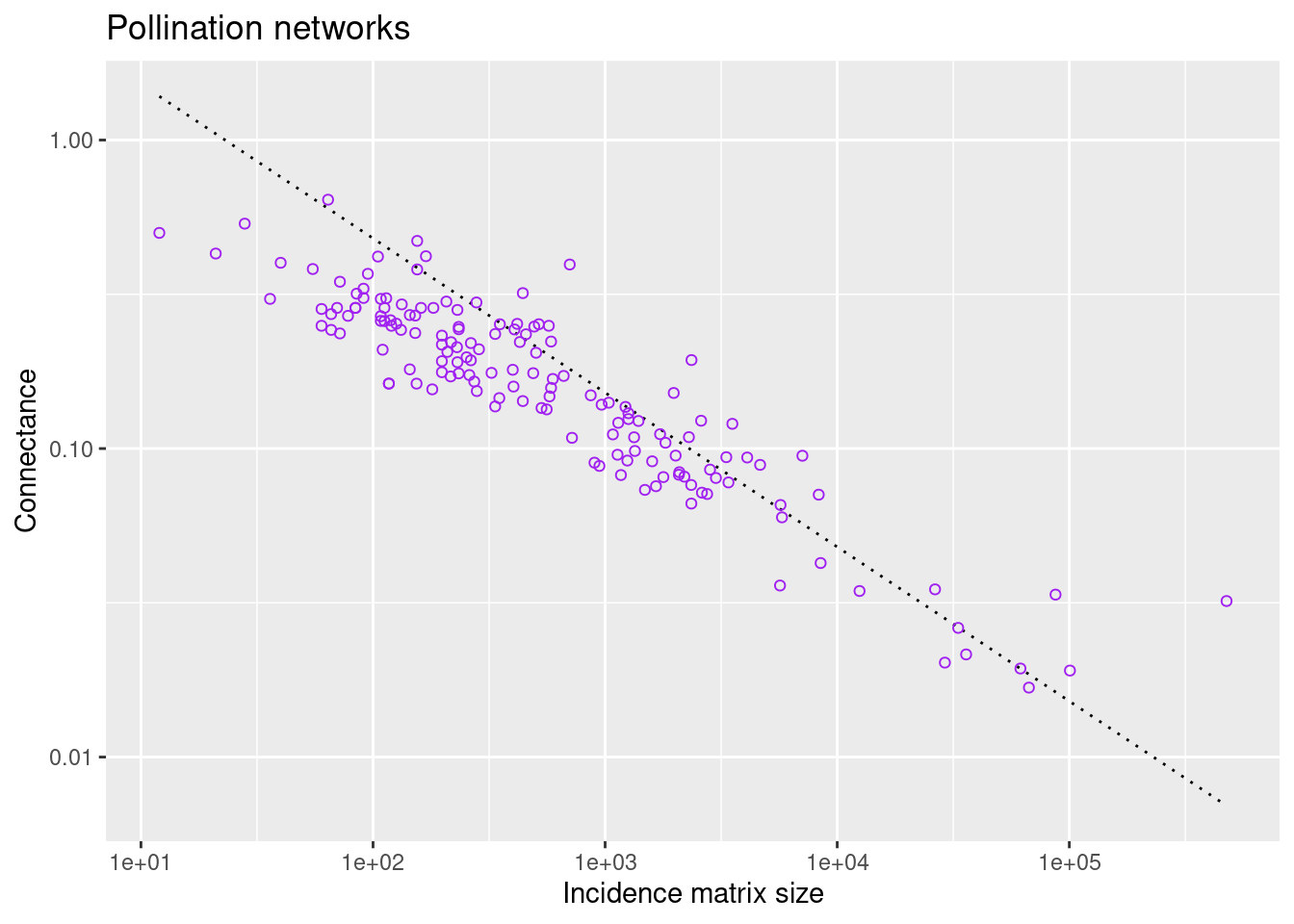 

The dotted line is a guide to the eye that corresponds to a power-law decay (note the log-log scale).

3.2 Filter by latitude

Making use of the information contained in the metadata, you can filter the networks by the latitude and longitude of the location in which the data was collected.
Assume you would like to display with a different color the connectance of the subset of networks in the tropical area. We start downloading the metadata of all networks in Web of life (see above)

nws_info <- read.csv(paste0(base_url,"get_network_info.php")) 
my_nws_info <- select(nws_info, network_name, location, latitude,longitude)

From this dataframe we select the names of networks recorded in the tropical region, namely in the area with latitude between -23.43647\(^\circ\) and 23.43647\(^\circ\).

tropical_nws_info <- nws_info %>% filter(.,between(latitude, -23.43647, 23.43647))  
tropical_nw_names <- distinct(tropical_nws_info, network_name) 

Now we keep in the dataframe pol_connectance_df only the data corresponding to tropical networks. In practice, we look for the intersection of the two ensembles: polination networks and tropical networks

tropical_pol_conn_df <- filter(pol_connectance_df, network_name %in% tropical_nw_names$network_name) %>%
  select(network_name, size, connectance)

At this point we can superimpose the (orange) points calculated for tropical networks to the previous plot

options(repr.plot.width=5, repr.plot.height=4)
ggplot() +
  ggtitle("Tropical pollination networks") +
  stat_function(fun = function(x) power_decay(x,4.,0.5), color ="black", linetype = "dotted") +
  geom_point(data = pol_connectance_df, aes(size, connectance), color = "purple", shape=1) +
  geom_point(data = tropical_pol_conn_df, aes(size, connectance), color = "dark orange") +
  labs(x = "Incidence matrix size", 
       y = "Connectance") +
  scale_x_continuous(trans='log10') +
  scale_y_continuous(trans='log10')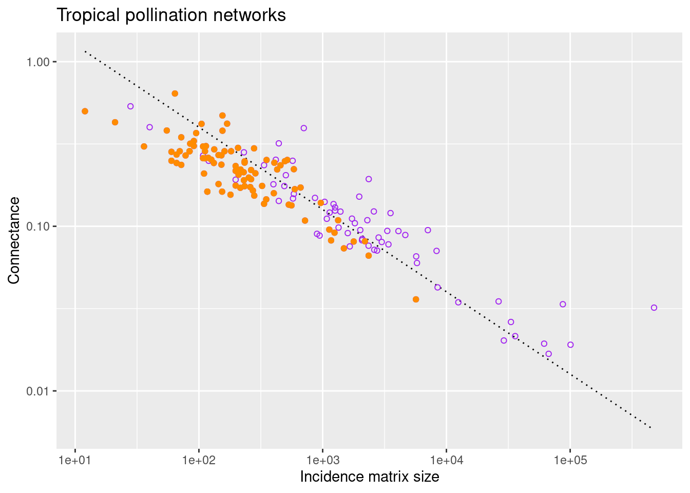 

3.3 Foodwebs

For foodwebs the connectance is defined as \[\begin{equation} \frac{2 \times n_l}{N \times (N-1)} \end{equation}\] where \(N\) is the number of species in the foodweb and \(n_l\) is the number of links. Referring to the example given in section 2.3 and relative commands, the connectance of the foodweb FW_002 is obtained as

links <- FW_002_nw %>% nrow() 
size <- nrow(adj_matrix)
conn <- 2*links/(size*(size-1))      
conn

## [1] 0.4175824