2 Analyze networks with igraph

In the language of graph theory (or complex networks) species of an ecological network would be the nodes (vertices) of a graph and links (or edges) their pairwise interactions.

The reference package for graph/network analysis is igraph. It is an open source software, optimized by professional developers and can be invoked from R, Python, Mathematica, and C/C++. The recommendation is that, whenever you need to do some operation or calculation with networks, you first look if that functionality is already provided in igraph. If not, you can probably build on some existing functions to develop your own function/package.

In the following we will use the word graph meaning an igraph object in the context of the igraph package. But, obviously, graph refers to a more general mathematical entity. Network data can be represented in several ways, corresponding to different data structures (classes). Below we will consider the following ones:

representation	data structure
edge list	dataframe
graph	igraph object
adjacency matrix	matrix/array
incidence matrix	matrix/array

2.1 From dataframe to igraph object

The network data downloaded from Web of life are stored in a representation (network_name, species1, species2, connection_strength). The last three columns correspond to the edgelist representation of a graph. Therefore, the values contained in those three columns can be converted into a graph object using the function graph_from_data_frame() of the igraph package

# download the foodweb FW_001 
json_url <- paste0(base_url,"get_networks.php?network_name=FW_001")
FW_001_nw <- jsonlite::fromJSON(json_url)

# check the class 
class(FW_001_nw)

## [1] "data.frame"

# import the igraph package (if not done at the beginning) 
library(igraph)

# select the 3 relevant columns and create the igraph object 
FW_001_graph <- FW_001_nw %>% select(species1, species2, connection_strength) %>% 
  graph_from_data_frame(directed = TRUE)

# check the class 
class(FW_001_graph)

## [1] "igraph"

As you can see from the last command, we have just created an igraph object. Note that, since in foodwebs it is relevant who eats whom, the representative graph is directed. This is specified setting the corresponding parameter as TRUE in the function graph_from_data_frame().

2.2 Plot a foodweb as a directed graph

Once the network is represented as an igraph object it can easily be visualized

plot(FW_001_graph, vertex.size=4, 
     vertex.label=NA, 
     edge.arrow.size= 0.3, 
     layout = layout_on_sphere)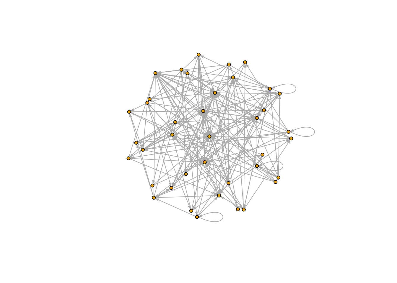

Other possible layouts are: layout_nicely, layout_with_kk, layout_randomly, layout_in_circle, layout_on_sphere.

2.3 From igraph object to adjacency matrix

Another way to represent an ecological network is the adjacency matrix, that is a square matrix whose rows and columns run over all the species name in the network and whose elements indicate the strength of interaction between species pairs (zero means no interaction). This data structure is generally less efficient from the perspective of memory storage w.r.t. an edge list, but it can be useful to facilitate visualization or to perform some calculations (e.g., evaluate the nestedness of a network, perform spectral analysis, etc.).

Using the function as_adjacency_matrix() of the igraph package the adjacency matrix associated with a given network can be created. Let us focus on the relatively small FW_002 foodweb. Some care must be put in passing the right arguments to the function as_adjacency_matrix()
because the graph is directed. The reader is addressed to the user manual for more details.

# download the foodweb FW_002
json_url <- paste0(base_url,"get_networks.php?network_name=FW_002")
FW_002_nw <- jsonlite::fromJSON(json_url)

# select the 3 relevant column and pass and create the igraph object 
FW_002_graph <- FW_002_nw %>% select(species1, species2, connection_strength) %>% 
  graph_from_data_frame(directed = TRUE)

# convert the igraph object into adjacency matrix 
adj_matrix <- as_adjacency_matrix(FW_002_graph, 
                                     type = "lower", # it is directed!!!
                                     attr = "connection_strength",
                                     sparse = FALSE)

If you give a quick look at the variable adj_matrix running the command

 head(adj_matrix)

you will notice that it does not produce exactly what we want:
1. elements are strings, instead of numerical values
2. there are some empty strings to indicate that a pair of species do not interact.
We can fix both problems as follows

# convert elements into numeric values 
class(adj_matrix) <-"numeric"

# remove NA values (previous empty strings)
adj_matrix[which(is.na(adj_matrix) == T)]<-0

# check dimensions and compare with the number of species on the Web interface 
dim(adj_matrix)

## [1] 14 14

# convert the adjacency matrix into a dataframe just for visualization purposes 
df <- adj_matrix %>% as.data.frame() 

df <- df[order((rownames(df))),] # to order by column names 

# visualize the adjacency matrix 
df %>% formattable()

	Leporinus friderici	Astyanax altiparanae	Hoplias malabaricus	Terrestrial Invertebrates	Astyanax fasciatus	Brycon nattereri	Hypostomus strigaticeps	Salminus hilarii	Zooplankton
Astyanax altiparanae	0.000	0.0000	0.500	0.0	0.000	0.000	0	0.740	0.0
Astyanax fasciatus	0.000	0.0000	0.100	0.0	0.000	0.000	0	0.060	0.0
Brycon nattereri	0.000	0.0000	0.000	0.0	0.000	0.000	0	0.115	0.0
Detritus	0.000	0.0000	0.001	0.3	0.000	0.003	1	0.000	0.6
Detritus Animal	0.010	0.0006	0.001	0.0	0.307	0.001	0	0.000	0.0
Hoplias malabaricus	0.000	0.0000	0.030	0.0	0.000	0.000	0	0.000	0.0
Hypostomus strigaticeps	0.000	0.0000	0.000	0.0	0.000	0.000	0	0.010	0.0
Import	0.252	0.0290	0.000	0.5	0.000	0.219	0	0.000	0.0
Leporinus friderici	0.000	0.0000	0.000	0.0	0.000	0.000	0	0.050	0.0
Macrophytes	0.100	0.1000	0.007	0.2	0.500	0.036	0	0.000	0.0
Phytoplankton	0.004	0.0200	0.000	0.0	0.001	0.000	0	0.000	0.4
Salminus hilarii	0.000	0.0000	0.000	0.0	0.000	0.000	0	0.000	0.0
Terrestrial Invertebrates	0.634	0.8500	0.361	0.0	0.192	0.742	0	0.025	0.0
Zooplankton	0.000	0.0000	0.000	0.0	0.000	0.000	0	0.000	0.0

2.4 Bipartite networks

Several ecologically relevant networks are bipartite, that is
1. interactions are not directed
2. species can be split in two groups and interactions occurs only from one group to the other.

Typical examples are pollination or seed-dispersal networks. Let us see how these features of bipartite networks affect the way in which their data has to be handled with igraph.
We first download the seed-dispersal network M_SD_002 and convert it into an igraph object:

# download the foodweb FW_002
json_url <- paste0(base_url,"get_networks.php?network_name=M_SD_002")
M_SD_002_nw <- jsonlite::fromJSON(json_url)

# select the 3 relevant columns and create the igraph object 
M_SD_002_graph <- M_SD_002_nw %>% select(species1, species2, connection_strength) %>% 
  graph_from_data_frame()

To turn this object into a bipartite graph, one needs to determine which nodes (species) of the graph M_SD_002_graph belong to one or the other guild, e.g., plants or animals.
Within each network we label species acting as resources and oppose them to the consumers. Technically, this information is returned by the boolean is.resource when the endpoint https://www.web-of-life.es/get_species_info.php is hit. For clearness, let us store this information in the list isResource

M_SD_002_info <- read.csv(paste0(base_url,"get_species_info.php?network_name=M_SD_002"))
isResource <- M_SD_002_info$is.resource %>% as.logical() # 0/1 converted to FALSE/TRUE

This list can be used to split the nodes of the graph M_SD_002_graph into two ecologically meaningful guilds; igraph uses the type (TRUE/FALSE) attribute of nodes to identify the two groups of species. In code, this reads

# Add the "type" attribute to the vertices of the graph 
V(M_SD_002_graph)$type <- !(isResource)

When representing a graph – M_SD_002_graph in this case – as an incidence matrix, we will adopt the convention that resources be associated with rows. These species are label with is.resource=TRUE. Instead, igraph displays as rows of the incidence matrix nodes with the attribute type=FALSE. For this reason, we applied the negation operator !() in the previous chunk.

One can also check that the igraph object was successfully converted into a bipartite graph running the following command

# check if igraph understands this object as bipartite 
is_bipartite(M_SD_002_graph)

## [1] TRUE

Since interactions are not directed it is appropriate to remove the arrows attribute from the links of our graph

E(M_SD_002_graph)$arrow.mode = "-"

Moreover, we would like to visualize our network assigning distinct colors to nodes belonging to different groups

V(M_SD_002_graph)$color <- ifelse(V(M_SD_002_graph)$type == TRUE, "lightblue", "lightgreen")

plot(M_SD_002_graph, 
     layout=layout_as_bipartite, 
     arrow.mode=0,
     vertex.label=NA,
     vertex.size=4,
     asp=0.2)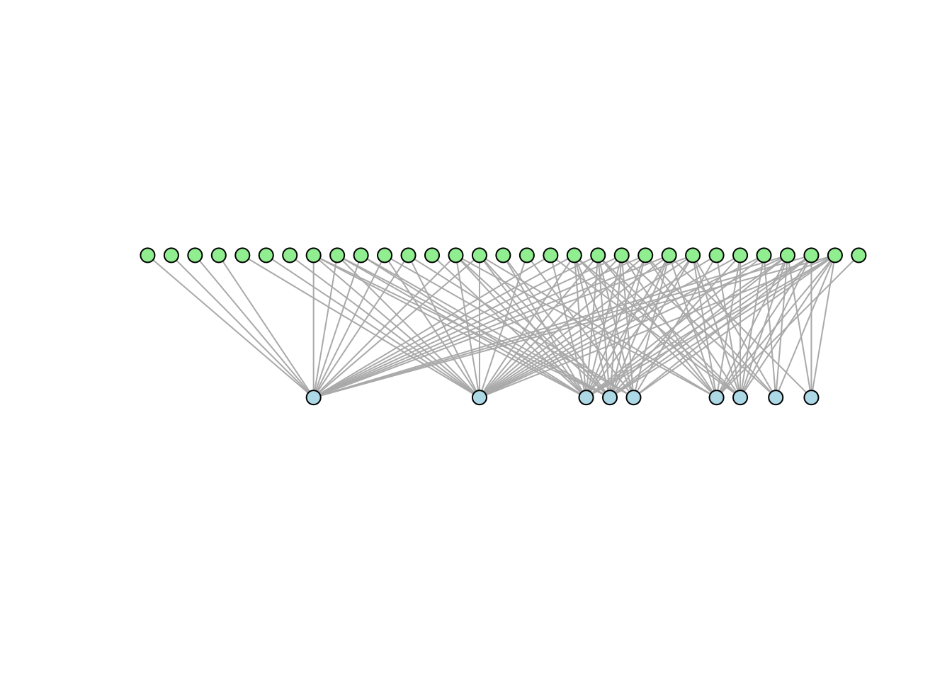

In the example above, the nodes of the top layer in the graph above represent plants while seed dispersers are displayed on the bottom layer. To adjust the distance between nodes one can play with their size (vertex.size) and the attribute asp of iplot.graph, which controls how rectangular a plot is: asp < 1 yields a wide plot, asp > 1 a tall plot.

From bipartite graph to incidence matrix

It is possible to pass from the representation of a bipartite graph to that of incidence_matrix. The latter is a matrix whose rows represent one group of species (e.g. plants) and columns the other group (e.g. animals). This can be achieved using the function as_incidence_matrix() of the igraph package. Mutatis mutandis we first repeat the same steps done for the conversion from an igraph object to adjacency matrix

# convert the igraph object into incidence matrix 
inc_matrix <- as_incidence_matrix(
  M_SD_002_graph,
  attr = "connection_strength",
  names = TRUE,
  sparse = FALSE
)

# convert elements into numeric values 
class(inc_matrix) <-"numeric"

# remove NA values (previous empty strings)
inc_matrix[which(is.na(inc_matrix) == T)]<-0

# check dimensions and compare with the number of species on the Web interface 
dim(inc_matrix)

## [1] 31  9

We can now visualize the elements of the incidence matrix with the function formattable() and order alphabetically rows and columns by relative names:

# convert the incidence matrix into a dataframe just for visualization purposes 
df <- inc_matrix %>% as.data.frame() 

df <- df[,order((colnames(df)))] # to order by column names 
df <- df[order((rownames(df))),] # to order by row names 

# visualize the incidence matrix 
df %>% formattable()

	Diphyllodes magnificus	Epimachus albertisii	Lophorina superba	Manucodia chalybatus	Manucodia keraudrenii	Paradisaea raggiana	Paradisaea rudolphi	Parotia lawesii	Ptiloris magnificus
Aglaia sp1 M_SD_002	0	0	0	0	0	3	0	1	0
Aporusa sp1 M_SD_002	0	0	1	0	0	0	0	0	0
Canthium sp1 M_SD_002	1	0	0	0	0	0	0	0	0
Chisocheton sp1 M_SD_002	13	5	23	1	7	13	3	10	16
Cissus aristata	1	0	0	1	0	0	0	0	0
Cissus hypoglauca	4	1	1	0	13	5	3	2	1
Dysoxylum sp1 M_SD_002	12	0	0	0	1	17	0	1	0
Elmerrillia sp1 M_SD_002	12	1	2	1	8	2	0	2	0
Endospermum sp1 M_SD_002	15	0	9	0	2	2	0	2	0
Ficus 181	0	0	0	0	7	0	1	2	0
Ficus 202	1	0	0	1	2	0	0	0	0
Ficus 217	0	0	0	0	9	0	0	0	0
Ficus 246	2	0	0	1	4	0	0	0	0
Ficus 275	5	0	2	8	40	13	4	1	0
Ficus 371	0	1	4	1	6	3	7	4	0
Ficus drupacea	0	0	0	0	2	0	0	0	0
Ficus gul	8	0	1	25	155	45	1	12	0
Ficus odoardi	8	0	1	19	55	20	0	6	2
Gastonia sp1 M_SD_002	58	0	0	0	17	24	3	22	7
Glochidion sp1 M_SD_002	1	0	0	0	0	0	0	0	0
Homalanthus sp1 M_SD_002	104	0	17	0	4	75	23	10	8
Myristica sp1 M_SD_002	1	0	0	0	3	1	0	3	0
Pandanus sp1 M_SD_002	5	0	2	0	0	2	1	0	0
Piper sp1 M_SD_002	0	0	0	0	1	0	0	0	0
Schefflera sp1 M_SD_002	2	0	0	0	0	0	10	47	1
Sloanea aberrans	2	0	0	0	0	0	0	0	0
Sloanea sogerensis	4	0	2	0	2	1	0	2	0
Sterculia sp1 M_SD_002	0	0	0	0	0	0	0	1	0
Syzygium sp1 M_SD_002	0	0	0	0	8	1	0	1	0
Uvaria sp1 M_SD_002	0	0	0	0	2	0	0	0	0
Zingiberaceae sp1 M_SD_002	2	0	0	1	0	0	1	0	0