4 Anaylize networks with bipartite
The
bipartite package offers several powerful tools for the analysis of
bipartite networks.
As a preliminary step to integrate Web of life with this package, one needs to convert network data into a bipartite graph (see Section 2.4).
For instance, after having downloaded and converted the relative data into an incidence matrix, one can visualize the network M_SD_002 using the function plotweb() the bipartite package:
# import the bipartite package (if not done at the beginning)
library(bipartite)
plotweb(inc_matrix)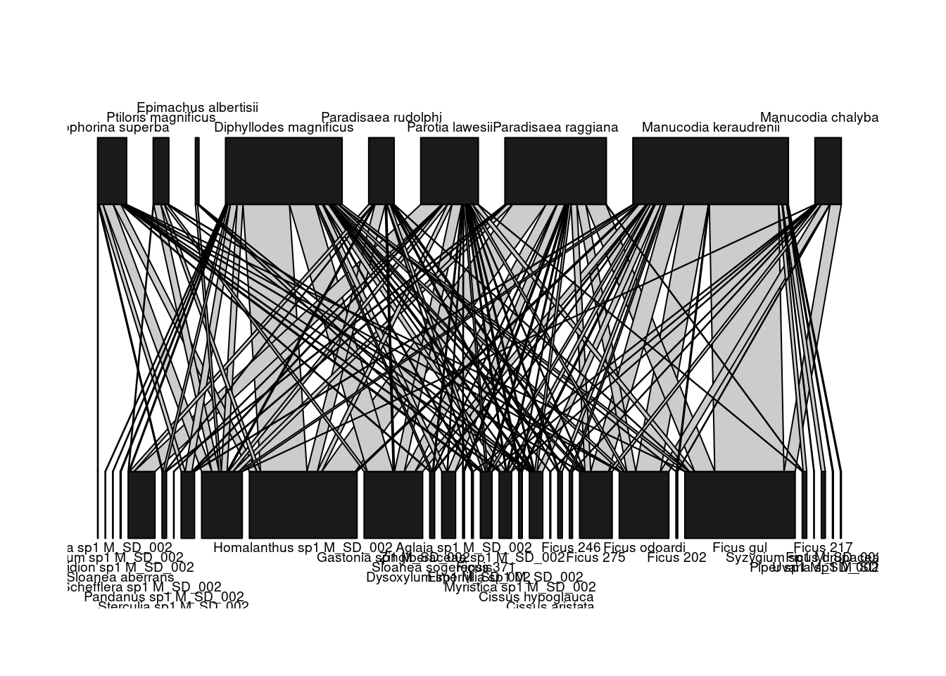
The two groups of species within this bipartite network are shown on different layers: seed dispersers (top) and plants (bottom).
Bipartite also offer also the the function visweb() to visualize the incidence matrix:
visweb(inc_matrix)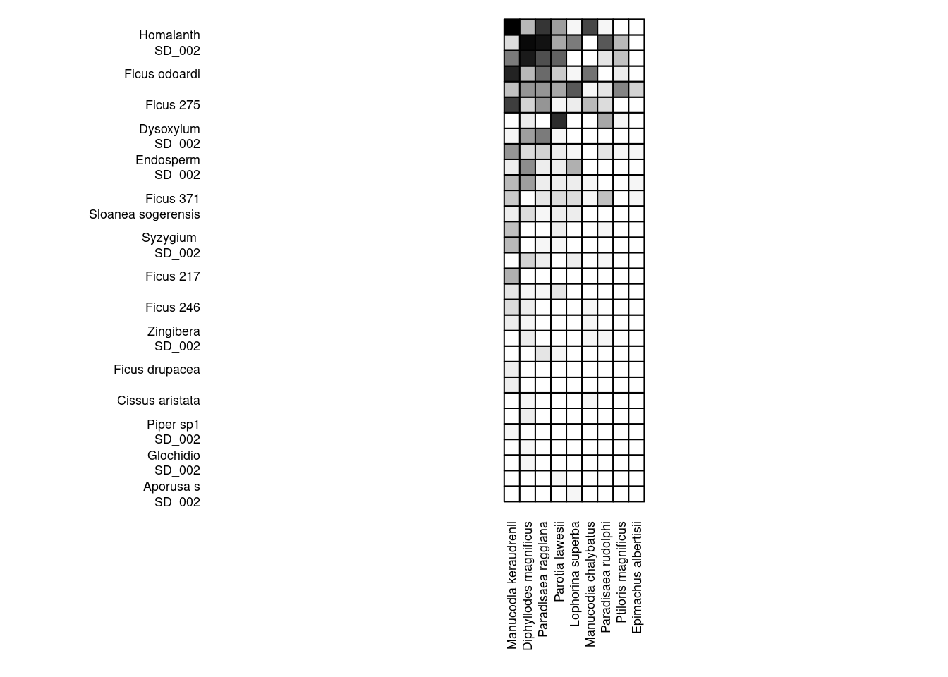
4.1 Network-level indices
Among other network properties, some indices characterizing an entire network can be computed calling the function networklevel() of the
bipartite package.
Here we just focus on the connectance.
The definition of connectance given at the beginning of Chapter 3 can be generalized to any bipartite network replacing:
plants \(\Rightarrow\) resources
animals \(\Rightarrow\) consumers
According to our convention, resources correspond to the rows of the incidence matrix while consumers to the columns. Counting the number of links, rows, and columns of the incidence matrix the connectance can readily be estimated.
Alternatively, one can obtain this index calling the function networklevel().
It is instructive to show how the connectance of the bipartite networks present in Web of life (i.e., all but foodwebs) can be computed with both approaches. In code, this is done as follows
base_url <- "https://www.web-of-life.es/"

# download all the networks
json_url <- paste0(base_url,"get_networks.php")
all_nws <- jsonlite::fromJSON(json_url)
head(all_nws)

# create a list of networks names filtering out food-webs
nw_names <- distinct(all_nws, network_name) %>%
  dplyr::filter(., !(network_name %like% "FW_"))

# initialize dataframe to store results
connectance_df <- NULL

for (nw_name in nw_names$network_name){

  nw <- filter(all_nws, network_name == nw_name)
  links <- nw %>% nrow()

  # select the 3 relevant columns and create the igraph object
  my_graph <- nw %>% select(species1, species2, connection_strength) %>%
    graph_from_data_frame(directed = FALSE)

  inc_matrix <- from_wol_graph_to_incidence_matrix(base_url, nw_name, my_graph, inc_matrix)

  nw_prop_bipartite <- networklevel(inc_matrix,
                                    index=c("connectance"),
                                    SAmethod="log")

  resources_num <- nrow(inc_matrix)
  consumers_num <- ncol(inc_matrix)
  conn <- links/(resources_num*consumers_num)

  connectance_row <- data.frame(nw_name,
                               resources_num,
                               consumers_num,
                               conn,
                               nw_prop_bipartite["connectance"])

  connectance_df <- rbind(connectance_df, connectance_row)

  print(paste0("connectance of ", nw_name, " network"))
}

rownames(connectance_df) <- NULL
colnames(connectance_df) <- NULL
colnames(connectance_df) <- c("network_name",
                             "num_resources",
                             "num_consumers",
                             "connectance",
                             "bipartite_connectance")
where we have gathered all the commands to convert the igraph object my_graph into a bipartirte graph and, subsequently, into
an incidence matrix within the function from_wol_graph_to_incidence_matrix(), which reads
from_wol_graph_to_incidence_matrix <- function(base_url, nw_name, wol_graph, inc_mat){

  # get info about species
  my_info <- read.csv(paste0(base_url,"get_species_info.php?network_name=",nw_name))

  isResource <- my_info$is.resource %>% as.logical() # 0/1 converted to FALSE/TRUE

  # Add the "type" attribute to the vertices of the graph
  V(wol_graph)$type <- !(isResource)

  # convert the igraph object into incidence matrix
  inc_mat <- as_incidence_matrix(
    wol_graph,
    attr = "connection_strength",
    names = TRUE,
    sparse = FALSE
  )

  # convert elements into numeric values
  class(inc_mat) <-"numeric"

  # remove NA values (previous empty strings)
  inc_mat[which(is.na(inc_mat) == T)]<-0

  return(inc_mat)
}
The reader can appreciate the perfect agreement between the two approaches running the command below.
connectance_df %>% formattable()To let the function networklevel() return multiple indices, one has to pass them to the index argument as a vector:
networklevel(inc_matrix, index=c("connectance", "nestedness","weighted nestedness","compartment diversity","Shannon diversity"), SAmethod="log")The reader is addressed to the bipartite manual to get more information about the network properties that can be computed using this package and about their definitions.